
QuickHelper
$20/per page/
Question description
┬Ā
*** You can use any statis tic software to solve (SPSS, Eviews, R...)
*** The result of each problem must contain RESULT TABLE (from the software) and EXPLANATION (Short or long)
*** The data file is in .xls form (Excel needed)
Background
A good understanding of the macroeconomic cycle with alternating recession and expansion periods (also known as the business cycle) is important for various decision makers. Macroeconomic policy is often based on predictions of this cycle, and such predictions can in’¼éuence investment decisions of large companies. Central banks and other institutions often publish so-called leading indicators that are helpful to predict the state of the economy. These indicators are based on macroeconomic series like job formation, interest rates, credit, demand, and supply.
In this case project you will predict GDP growth by using quarterly data on a hypothetical economy from 1950 quarter 1 to 2015 quarter 4. The data set contains the GDP of the economy and two leading indicators li1 and li2. In order to evaluate the predictive performance of econometric models, you need to split the data in two parts. As estimation sample you take the period from 1951 to 2010 (240 observations), and as evaluation sample you take the period from 2011 to 2015 (20 observations). The ’¼ürst year of data (1950) is used only to create lags of variables.
The project consists of two parts. In the ’¼ürst part (a-c) you use logit models to predict whether the economic situation improves or declines, and in the second part (d-g) you use time series models to predict the size of the growth rate of the economy.
Data
The data ’¼üle Case GDP contains the following variables:
ŌĆó DATE: Date of the observation;
ŌĆó GDP: Gross Domestic Product of the economy;
ŌĆó GDPIMPR: dummy variable indicating whether the GDP has increased (1) or decreased (0);
ŌĆó LOGGDP: Log of Gross Domestic Product;
ŌĆó GrowthRate: Relative growth of the economy: GrowthRatet = log(GDPt ) ŌłÆ log(GDPtŌłÆ1);
ŌĆó li1: First leading indicator;
ŌĆó li2: Second leading indicator;
ŌĆó T: Linear trend (where the ’¼ürst observation, for 1950 quarter 1, is de’¼üned as 0).
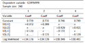
(a) The table below summarizes the outcomes of four logit models to explain the direction of economic development
(GDPIMPR) for the period 1951 to 2010. Perform three Likelihood Ratio tests to prove both the individual and
the joint signi’¼ücance of the 1-quarter lags of li1 and li2, where the alternative hypothesis is always the model
with both indicators included. (Please see image name TABLE 1)
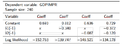
b) It could be that the leading indicators lead the economy by more than 1 quarter. The table below summarizes
outcomes of four logit models that di’¼Ćer in the lags of the indicators. For what reason can we use McFadden
R2 to select the best lag structure among these four models? Compute the four values of McFadden R2 (with
four decimals) and conclude which model is optimal according to this criterion. (Please see image name TABLE 2)
(c) Use the logit model 3 of part (b) (with li1(-2) and li2(-1)) to calculate the predicted probability of economic
growth for each of the 20 quarters of the evaluation sample. Assess the predictive performance by means of
the prediction-realization table and the hit rate, using a cut-o’¼Ć value of 0.5. Evaluate the outcomes.
(d) Perform the Augmented Dickey-Fuller test on LOGGDP to con’¼ürm that this variable is not stationary. Use only
the data in the estimation sample and include constant, trend, and a single lag in the test equation (L = 1,
see Lecture 6.4). Present the coe’¼ācients of the test regression and the relevant test statistic, and state your
conclusion.
(e) Consider the following model: GrowthRatet = ╬▒ + ŽüGrowthRatetŌłÆ1 + ╬▓1li1tŌłÆk1 + ╬▓2li2tŌłÆk2 + ╬Ąt . Here the
numbers k1 and k2 denote the lag orders of the leading indicators. Estimate four versions of this model on the
estimation sample from 1951 to 2010, by setting k1 and k2 equal to either 1 or 2. Show that the model with
k1 = k2 = 1 gives the largest value for R2, and present the four coe’¼ācients of this model in six decimals.
(f) Perform the Breusch-Godfrey test for ’¼ürst-order residual serial correlation for the model in part (e) with k1 =
k2 = 1. Does the test outcome signal misspeci’¼ücation of the model?
(g) Use the model in part (e) with k1 = k2 = 1 to generate a set of twenty one-step-ahead predictions for the
growth rates in each quarter of the period 2011 to 2015. Note that the required values of the lagged leading
indicators are available for each of these forecasts. Calculate the root mean squared error of these forecasts
and present a time series graph of the predictions and the actual growth rates.
Attachments: